"To deal with hyper-planes in a 14 dimensional space, visualize a 3D space and say 'fourteen' very loudly. Everyone does it." - Geoff Hinton

Overview

HyperTools is designed to facilitate dimensionality reduction-based visual explorations of high-dimensional data. The basic pipeline is to feed in a high-dimensional dataset (or a series of high-dimensional datasets) and, in a single function call, reduce the dimensionality of the dataset(s) and create a plot. The package is built atop many familiar friends, including matplotlib, scikit-learn and seaborn. Our package was featured in 2017 on Kaggle's now-retired "No Free Hunch" blog (archived copy). For a general overview, you may find this talk useful (given as part of the MIND Summer School at Dartmouth).

What's new in 1.0

HyperTools 1.0 modernizes the toolbox while keeping the familiar API:

• Interactive plotting (optional): hyp.plot(..., backend='plotly') renders interactive figures. With the default backend='auto', HyperTools automatically uses plotly on Google Colab and Kaggle (where interactive figures work best and plotly is preinstalled) and matplotlib everywhere else — existing workflows are unchanged. The two backends produce visually matched output: identical colors, line/marker styles and sizes, format strings, and the signature cube/square framing.

• Multicolored lines: passing continuous values (or a per-observation matrix) as hue together with a line format colors each trajectory continuously along its length, on both backends.

• hyp.apply_model: a unified stack → fit-once → unstack core for applying any scikit-learn style model (or pipeline of models) across one or more datasets, with return_model=True for reuse on held-out data.

• Mixture-model ("soft") clustering: cluster and plot support GaussianMixture, BayesianGaussianMixture, LatentDirichletAllocation, and NMF. hyp.cluster returns per-observation membership proportions, and hyp.plot colors each observation by blending component colors according to its mixture weights.

• Richer coloring: the hue argument now accepts categorical labels, continuous values, or entire matrices (e.g. mixture proportions or model weights), which are mapped to colors via the new mat2colors helper (from hypertools.plot.colors import mat2colors).

• Nested-list input: hyp.plot([[a, b], [c]]) colors datasets by their outermost grouping and renders more deeply nested datasets with thinner, fainter lines.

• Hull surfaces (optional): hyp.plot(..., surface=True) overlays a smooth, lit surface over each dataset's convex hull — a filled outline in 2D, or a shaded, Taubin-smoothed "blob" in 3D. A dict of scalar options (e.g. surface={'alpha': 0.6}) customizes all surfaces at once; a list of bools/dicts (e.g. surface=[{'alpha': 0.2}, {'alpha': 0.8}]) controls alpha/color/lighting/smoothing per dataset.

• Morph animation: hyp.plot(datasets, animate='morph') treats each dataset as a point cloud and morphs smoothly between them (Hungarian- matched, smoothstep-eased), holding on each one along the way; rotations accepts a per-segment list for independent camera control over each hold and transition, and surface=True composes with it to morph a lit hull instead of raw points. See examples/plot_shape_morph.py and examples/animate_surface_morph.py.

• More animation styles, and 2-D animation: in addition to True/ 'parallel', animate='spin' keeps all the data drawn and spins the camera, 'serial' reveals each dataset one at a time in list order, and 'window' (hyp.plot(traj, animate='window', focused=2)) slides a fixed- length, fully-opaque window along each trajectory. Every style except 'spin' (which is inherently a 3-D camera move) now also works for ndims=2 data, using a fixed (non-rotating) viewport.

• hyp.Pipeline: a scikit-learn-style Pipeline chains manip/normalize/reduce/align/cluster stages, fit once and reused on new data without refitting -- hyp.plot(A, ..., return_model=True) returns a bundle whose 'pipeline' entry can be passed back in as hyp.plot(B, pipeline=bundle['pipeline']) to apply the exact same fitted transformation to a structurally-identical dataset B.

• hyp.manip and manip chaining: hyp.manip(data, model='ZScore') applies a manipulation (Normalize, ZScore, Smooth, Resample) to each dataset. Smooth and Resample run independently per dataset (kernels never cross dataset boundaries); ZScore and Normalize also transform each dataset separately but fit one shared set of statistics across all datasets in a list (like normalize='across'). A list of specs chains several manipulations as a Pipeline, and hyp.plot(data, manip=[...]) runs the chain at the canonical manip stage -- first, before normalize/reduce/align/cluster -- e.g. hyp.plot(data, manip=[{'model': 'Smooth', 'kwargs': {'kernel_width': 5}}, 'ZScore'], reduce='PCA').

• Autoencoder reducers (optional): hyp.reduce/hyp.plot(..., reduce= 'Autoencoder') supports six torch-backed autoencoder reducers (Autoencoder, DeepAutoencoder, SparseAutoencoder, ConvolutionalAutoencoder, SequenceAutoencoder, VariationalAutoencoder), gated behind pip install "hypertools[torch]".

• gensim text vectorizers/semantic models (optional): hyp.plot(texts, vectorizer='Word2Vec', semantic=None, reduce='PCA') (and hyp.tools.text2mat) add Word2Vec/Doc2Vec/FastText vectorizers and LdaModel/LsiModel/HdpModel semantic models, gated behind pip install "hypertools[gensim]" -- pass semantic=None with an embedding vectorizer like Word2Vec since the default LDA semantic stage rejects negative embedding values. Note that non-default vectorizers train on the default corpus='wiki' corpus the first time, which can take a couple of minutes even for tiny inputs; pass corpus= a list of your own documents to train on those instead.

• LSL streaming (optional): hyp.io.lsl_stream(type='EEG') resolves a live Lab Streaming Layer stream and wraps it for hyp.plot(..., stream_init=200, stream_chunk=20), gated behind pip install "hypertools[lsl]".

• hyp.predict/hyp.impute: hyp.predict(data, model='Kalman', t=10) forecasts t new rows continuing each dataset. Kalman, GaussianProcess, AutoRegressor, and ARIMA work with the base install (pykalman/statsmodels are core deps); Laplace needs pip install "hypertools[predict]" (skaters) and Chronos needs pip install "hypertools[predict-hf]". hyp.impute(data, model='PPCA') fills missing (NaN) values in place; the Kalman imputer also works with the base install. Both take return_model=True for reuse.

• Kaggle loader: hyp.load('kaggle/uciml/iris') downloads a public Kaggle dataset anonymously via kagglehub, gated behind pip install "hypertools[kaggle]".

• Density shading (optional): hyp.plot(..., density=True) overlays a subtle KDE "glow" behind the data (a 2D heatmap or 3D volumetric cloud) showing where each dataset's points concentrate; off by default.

• Colorbars: hyp.plot(..., colorbar=True) draws a colorbar matching whatever color mapping is already in use — a continuous gradient for a numeric hue, or a segmented, labeled bar for discrete groups/clusters.

• MultiIndex DataFrames: a DataFrame with a row MultiIndex is expanded automatically into one leaf trace per index combination plus a thicker, more opaque mean trace per level of grouping, colored by the top-level index value.

• Per-dataset animation trails: chemtrails/precog/bullettime each accept a list of bools (one per dataset) so different datasets in the same animation can show different trail styles, in addition to a single bool applied to all of them.

• More hyp.load sources: in addition to the built-in example datasets and local files, hyp.load now resolves Hugging Face dataset ids, Google Sheets/Drive links, Dropbox links, and arbitrary URLs, plus more local file formats (.npy/.npz, .csv/.tsv/.txt, .json, .parquet, .mat, .xlsx/.xls).

• Faster and cleaner: import hypertools is ~3.5x faster (heavy dependencies load lazily); plotting no longer mutates global matplotlib settings; the unreliable result cache was removed; HDBSCAN now comes from scikit-learn (no extra dependency); packaging follows current standards (pyproject.toml, Python 3.10–3.13).

• Retired legacy arguments: the long-deprecated group (use hue), model/model_params (use reduce), and align(method=...)/ align=True (use align='hyper') arguments were removed and now raise errors instead of being silently accepted. cluster's ndims= is no longer a standalone reduction step: it is only forwarded to the reduce= stage, and a warning fires if it is passed without reduce=. Legacy data: geo files saved by hypertools ≥0.8 (pickle-format) still load — the internal unpickle-only shim reads them and returns their raw data, with retired arguments translated or skipped with a warning on replay. Older pre-0.8 deepdish/HDF5-format geos cannot be read directly under HyperTools' required NumPy 2 (the deepdish reader is unmaintained and imports only under numpy<2); hyp.load detects them and raises a message explaining the one-time out-of-process conversion:

  # in a throwaway environment, convert an old .geo to a modern format once
  python -m venv /tmp/dd && /tmp/dd/bin/pip install "numpy<2" deepdish
  /tmp/dd/bin/python -c "import deepdish as dd, numpy as np; \
      d = dd.io.load('old.geo'); np.savez('old_converted.npz', \
      **{'data': np.asarray(d['data'], dtype=object)})"
  # then load old_converted.npz with hypertools as usual

Try it!

Check the repo of Jupyter notebooks from the HyperTools paper (note: those notebooks predate the 1.0 API described below). For up-to-date, runnable examples covering every 1.0 feature, see the example gallery in the docs.

Installation

To install the latest stable version run:

pip install hypertools

To install the latest unstable version directly from GitHub, run:

pip install -U git+https://github.com/ContextLab/hypertools.git

Or alternatively, clone the repository to your local machine:

git clone https://github.com/ContextLab/hypertools.git

Then, navigate to the folder and type:

pip install -e .

(These instructions assume that you have pip installed on your system)

Requirements

• python>=3.10
• scikit-learn>=1.4.0
• pandas>=2.2.0
• seaborn>=0.13.0
• matplotlib>=3.8.0
• scipy>=1.13.0
• numpy>=2.0.0
• umap-learn>=0.5.5, numba>=0.59
• pydata-wrangler>=0.5.1 (data-wrangling core)
• pykalman>=0.11, statsmodels>=0.14 (Kalman/ARIMA forecasting and imputation)
• requests, dill, ipympl
• ffmpeg (for saving animations)

All Python dependencies are declared in pyproject.toml and installed automatically by pip. The base install covers all core functionality (plotting, dimensionality reduction, alignment, clustering, normalization, and Kalman/ARIMA forecasting + imputation) and therefore pulls in the full scientific stack (NumPy, SciPy, pandas, scikit-learn, matplotlib, seaborn, UMAP/Numba, statsmodels, pykalman, ipympl, pydata-wrangler); it is not a minimal footprint. Heavier optional model families are separated into extras that add features on request (mix and match, e.g. pip install "hypertools[interactive,torch]"):

• interactive -- plotly + kaleido, for hyp.plot(..., backend='plotly'). Note: kaleido 1.x renders static images (PNG/PDF, and the frames of saved plotly animations) through a headless Chrome/Chromium, which it does not install. If image/GIF/video export from the plotly backend fails with a browser/Chromium error, install Chrome or Chromium (or run plotly_get_chrome). Interactive/HTML plotly output needs no browser.
• text -- transformer/sentence-transformers text embeddings (via datawrangler's hf extra)
• predict -- the skaters Laplace ensemble forecaster for hyp.predict (Kalman, GaussianProcess, AutoRegressor, and ARIMA already work with the base install)
• predict-hf -- the Hugging Face Chronos forecaster for hyp.predict
• io -- .xlsx support for hyp.load
• density3d -- smooth 3-D density=True iso-surfaces (scikit-image)
• torch -- the six autoencoder reducers (reduce='Autoencoder' and variants)
• kaggle -- hyp.load('kaggle/<owner>/<dataset>')
• lsl -- hyp.io.lsl_stream(...) (Lab Streaming Layer input)
• gensim -- Word2Vec/Doc2Vec/FastText vectorizers and LdaModel/LsiModel/HdpModel semantic models
• dev -- test/development dependencies (pip install -e ".[dev]")

Documentation

Check out our readthedocs page for further documentation, complete API details, and additional examples.

Citing

We wrote a short JMLR paper about HyperTools, which you can read here, or you can check out a (longer) preprint here. We also have a repository with example notebooks from the paper here.

Please cite as:

Heusser AC, Ziman K, Owen LLW, Manning JR (2018) HyperTools: A Python toolbox for gaining geometric insights into high-dimensional data. Journal of Machine Learning Research, 18(152): 1--6.

Here is a bibtex formatted reference:

@ARTICLE{heusser2018hypertools,
    author  = {Andrew C. Heusser and Kirsten Ziman and Lucy L. W. Owen and Jeremy R. Manning},    
    title   = {HyperTools: a Python Toolbox for Gaining Geometric Insights into High-Dimensional Data},    
    journal = {Journal of Machine Learning Research},
    year    = {2018},
    volume  = {18},	
    number  = {152},	
    pages   = {1-6},	
    url     = {http://jmlr.org/papers/v18/17-434.html}	
}

Contributing

If you'd like to contribute, please first read our Code of Conduct.

For specific information on how to contribute to the project, please see our Contributing page.

Testing

CI runs on every push via GitHub Actions (badge at the top of this page).

To test HyperTools locally, install pytest (pip install -e ".[dev]") and run pytest in the HyperTools folder.

Examples

See here for more examples.

Plot

import numpy as np
import hypertools as hyp

# two random-walk "datasets" (rows = observations, columns = features)
walk = lambda seed: np.cumsum(np.random.default_rng(seed).standard_normal((300, 10)), axis=0)
list_of_arrays = [walk(1), walk(2)]
list_of_labels = ['A'] * 300 + ['B'] * 300  # one label per observation

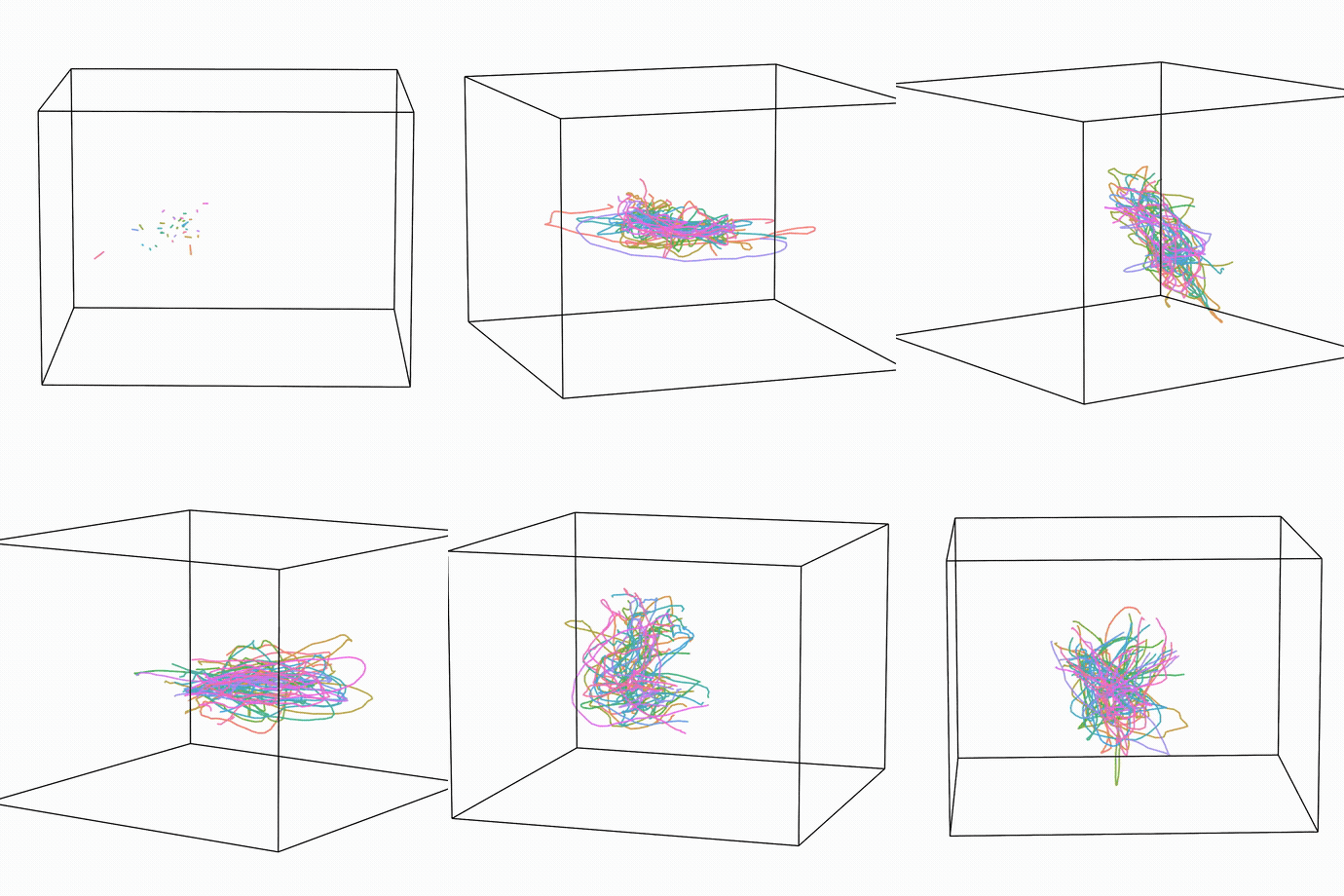
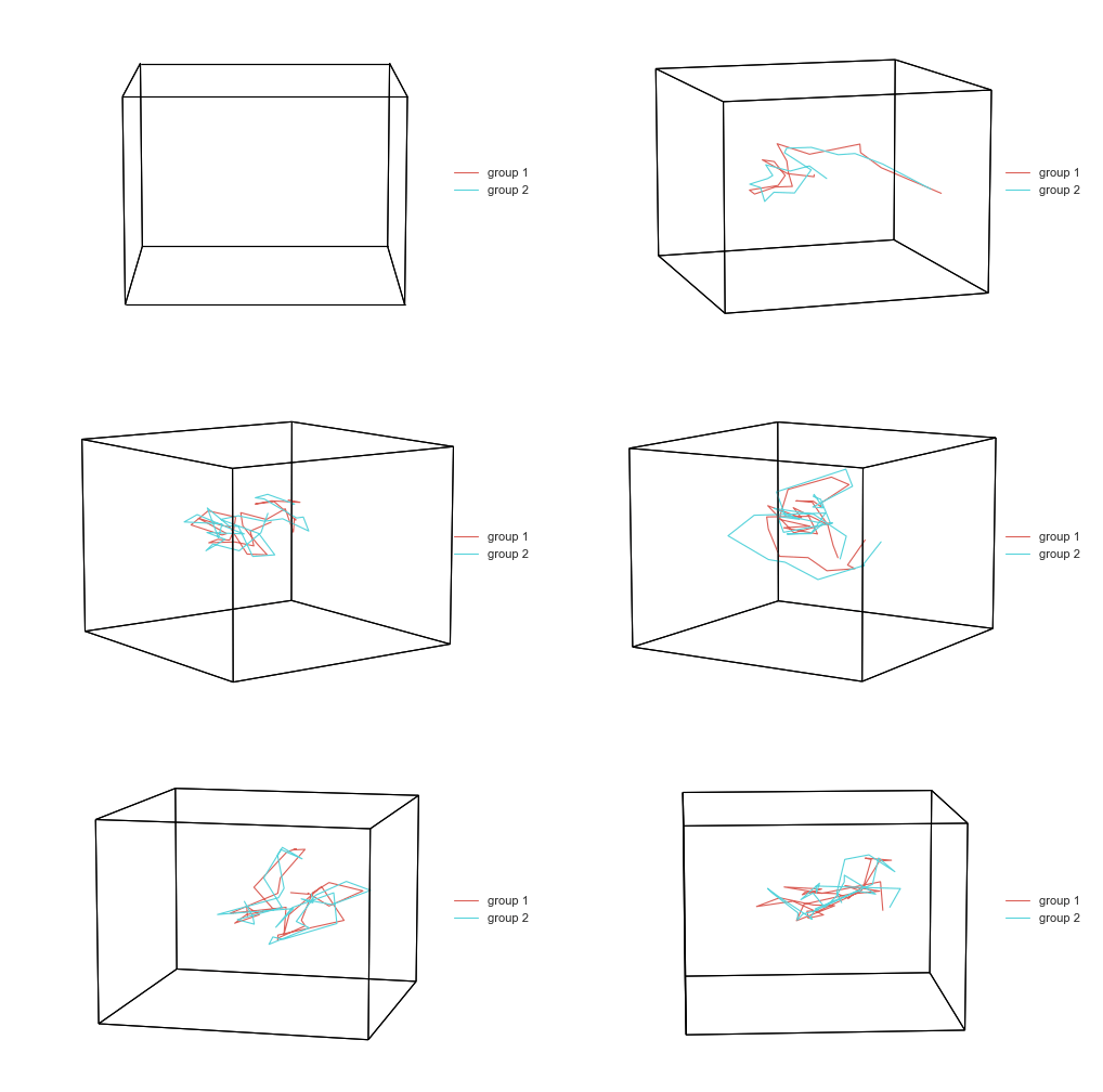
hyp.plot(list_of_arrays, animate=True, hue=list_of_labels)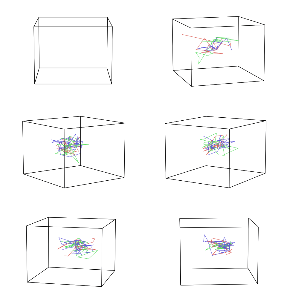

Align

import numpy as np
import hypertools as hyp

# rotated, noisy views of one shared trajectory
rng = np.random.default_rng(0)
base = np.cumsum(rng.standard_normal((300, 3)), axis=0)
list_of_arrays = [base @ np.linalg.qr(rng.standard_normal((3, 3)))[0]
                  + 0.05 * rng.standard_normal(base.shape) for _ in range(3)]

hyp.plot(list_of_arrays, align='hyper')

BEFORE

AFTER

Cluster

Soft ("mixture-model") clustering, new in 1.0 -- each point's color blends its component memberships:

import numpy as np
import hypertools as hyp

# three overlapping point clouds
rng = np.random.default_rng(0)
array = np.vstack([rng.standard_normal((100, 3)) + offset
                   for offset in ([0, 0, 0], [4, 0, 0], [0, 4, 0])])

hyp.plot(array, 'o', cluster='GaussianMixture', n_clusters=3)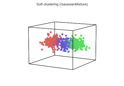

Surfaces

New in 1.0: overlay a smooth, lit surface over each dataset's convex hull:

import numpy as np
import hypertools as hyp

rng = np.random.default_rng(0)
blob_a = rng.standard_normal((100, 3))
blob_b = rng.standard_normal((100, 3)) + [4, 0, 0]

hyp.plot([blob_a, blob_b], '.', surface=True)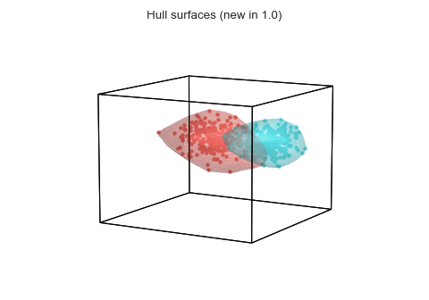

Describe

import numpy as np
import hypertools as hyp

rng = np.random.default_rng(0)
list_of_arrays = [np.cumsum(rng.standard_normal((200, 20)), axis=0)
                  for _ in range(3)]

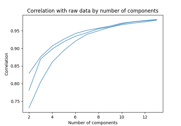
hyp.describe(list_of_arrays, reduce='PCA', max_dims=14)